Support Vector Machine

Author

Dr. Mohammad Nasir Abdullah

Support Vector Machine

Support vector machine (SVM) is a powerful supervised machine learning algorithm used for classification and regression tasks.

The objective of SVM is to find the optimal hyperplane that separates the datapoints into different classes or categories in the future space while maximixing the margin between the classes.

SVM is effective for binary classification problems but can be extended to handle multi-class classification and regression tasks.

Hyperplane

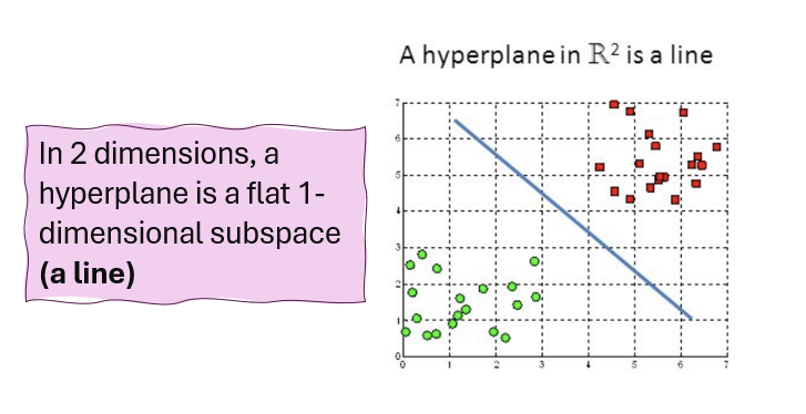
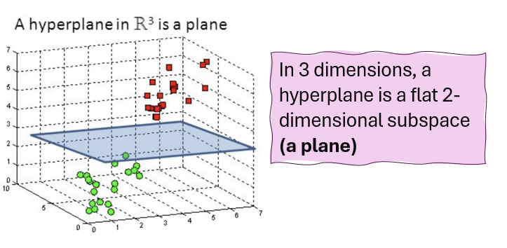
A flat affine subspace of dimension \(p-1\). A hyperplane is a decision boundary that separates the feature space into different regions corresponding to different classes.

In \(p>3\) dimensions, it can be hard to visualise a hyperplane, but the notion of a \(p-1\) -dimensional flat subspace still applies.

The mathematical definition of a hyperplane in \(p\)-dimensions:

\[ h(x)= \beta_{0}+\beta_{1}X_{1}+\beta_{2}X_{2}+...+\beta_{p}X_{p}=0 \]

Defines a \(p\)-dimensional hyperplane for a point \[X=(X_{1},X_{2},..,X_{1})^T\] in \(p\)-dimensional space.

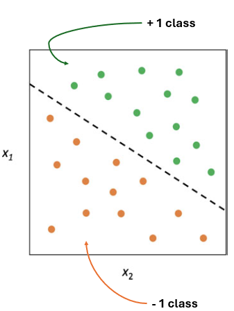
Suppose that \(X\) does not satisfy the equation but:-

\(y_{i} \times h(X)>0\) , then \(X\) lies on \(+1\) class (green), if \(y_{i} \times h(X)<0\) , then \(X\) lies on \(+1\) class (orange)

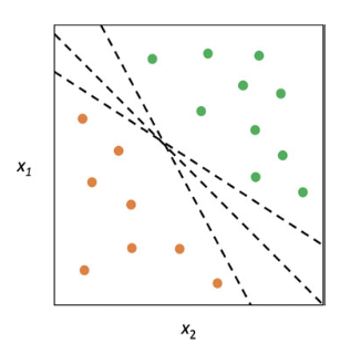
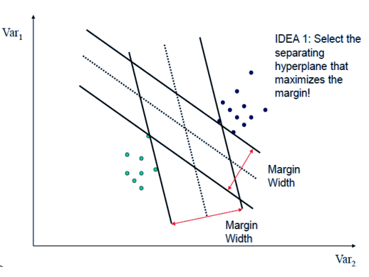
The separating hyperplane cannot be unique. One can define many separating hyperplane within the same dataset. To choose the “best” one (Maximal Margin Hyperplane), We can compute the perpendicular distance from each training observation or retain the smallest distance (called “margin”).
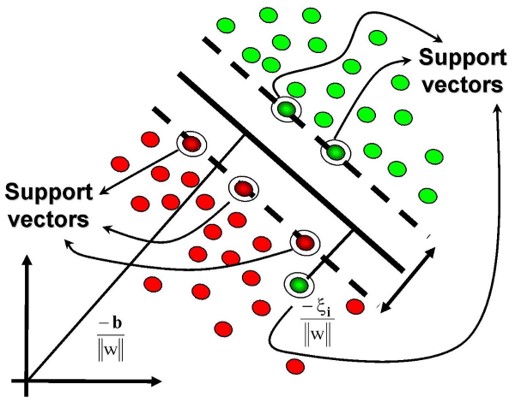
Maximal Margin

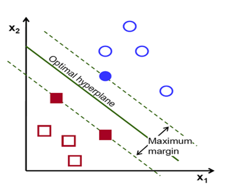
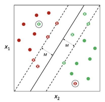
Maximal margin is the distance between the hyperplane and the nearest data point (support vector) from each class. The optimal hyperplane in SVM is the one that maximizes this margin, providing the largest separation or margin between the class.

Maximal Margin is the separating hyperplane for which the margin is largest. It is the hyperplane that has the largest minimum distance to the training observations.

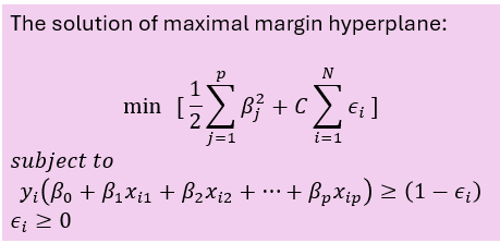
The maximal margin hyperplane is determined by searching the largest minimal distance between observation and the separating hyperplane. The solution of maximal margin hyperplane :

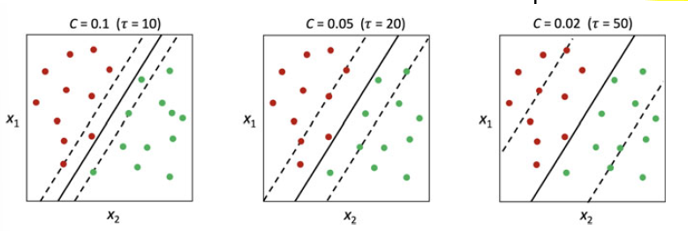
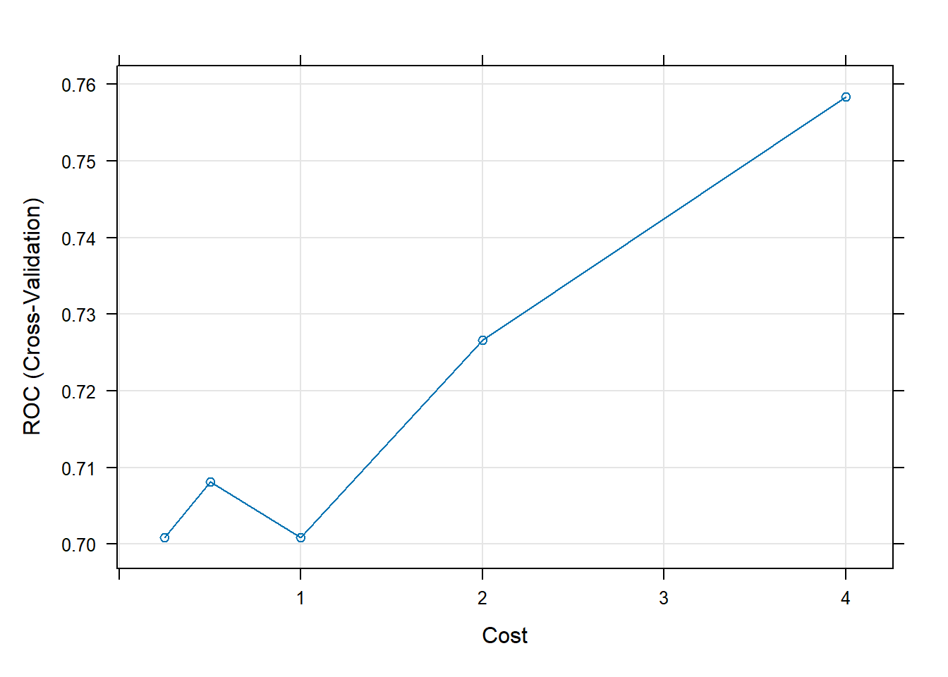
The penalization parameter \(C\) is equal to \(\frac{1}{\tau}\). It has a central role in classification performance. When \(C\) is larger, it produce tighter margins, When \(C\) is smaller, it produce wider margins. It is a trade-off between prediction variance and prediction bias.

Non-Separable Classes

If classes is non separable, a maximal margin hyperplane able to perfectly separate them simply does not exist. If classes are not separable, we would like to allow an observations to cross the boundaries provided by the marginal hyperplanes. Possibly allow for misclassification.

Solution: Provide larger robustness to specific configurations of the observations. Improving classification accuracy for the training observations.

There are 2 approaches to deal with non-separable class in the SVM:

  1. Feature polynomial expansion

  1. SVM with kernel adaptation

Kernels

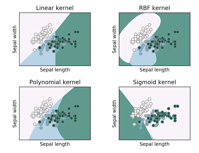
SVM utilises kernel functions to map the input data points into a higher dimensional space where the separation between the two classes becomes easier. This allows SVM to solve complex non-linear problem as well.

The SVM’s optimization for kernels:

where is the inner product between vector \(x\) and \(x_{i}\) and \(\alpha_{i}\) is a parameter specific to every observation \(i=1,2,3,...,N\) .

The \(<x, x_{i}>\) can be generalize to the nonlinear transformation using kernel transformation as follows:

\[ G(x)= \beta_{0}+\sum\alpha_{i}K(x,x_{i}) \]

where \(K(.)\) is kernel function.

There are two kernel transformation are generally used:

  1. Polynomial kernel

    \[ K(x,x_{i})=[1+\sum X_{ij} x_{i'j}]^d \]

    where \(d=1\) equivalent to linear support vector classifier.
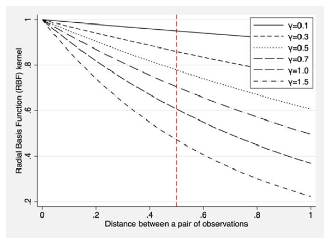
  2. Radial basis kernel

\[ K(x,x_{i})=exp[-\gamma\sum(x_{ij}-x_{i'j})^2] \]

it is a function of the Euclidean distance between the pair \(i\) and \(i'\) instead of the inner product.

The radial basis kernel behave similar to KNN (k-Nearest Neighbor) classifier. Choosing the right \(\gamma\) implying the sensitiveness of the classification. When \(\gamma\) is low, the classification becomes more sensitive to the distance, and larger distances can count a lot for the classification of a given test point. When \(\gamma\) is high, the classification become less sensitive to the distance and larger distances can count much less for classification (~ small \(k\) in \(k\)NN).

Advantages of SVM

  • Training is relatively easy

  • no local minima

  • It scales relatively well to high dimensional data

  • Trade-off between classifier complexity and error can be controlled explicitly via \(C\)

  • Robustness of the results

  • The “curse of dimensionality” is avoided.

Disadvantages of SVM

  • What is the best trade-off parameter \(C\)?

  • Need a good transformation of the original space.

Note!
  • Regularization parameter \(C\) that controls the trade-off between maximizing the margin and minimizing the classification error.

  • A smaller value of \(C\) allows for a wider margin and more misclassifications.

  • A larger value of \(C\) penalizes misclassifications more heavily, leading to a narrower margin.

Steps to perform SVM using Caret

Step 1: Loading Dataset
Step 2: Data Pre-Processing
Step 3: Splitting the dataset
Step 4: Performing Support Vector Machine classifier
Step 5: Model Prediction
Step 6: Model Evaluation
Step 7: Variable Importance

Example 1

Let’s revisit the Alzheimer’s disease dataset.

The Alzheimer’s disease (AD) Gene expression dataset from this link: https://sta334.s3.ap-southeast-1.amazonaws.com/Ready+for+Analysis.csv

The gene expression datasets of brain tissue was searched in the Gene Expression Omnibus (GEO) database using query: “Alzheimer* AND Homo sapiens” filtered by “Expression profiling by array” in August 2024. There are about 6,308 datasets found in search results. Out of these, 102 entries were sifted through. Finally, three datasets were chosen to be considered in this study since they were generated using the same platform (GSE5281, GSE48350, and GSE1297).

Step 1: Data loading

data1 <- read.csv("https://sta334.s3.ap-southeast-1.amazonaws.com/Ready+for+Analysis.csv")
head(data1)
    Group        PSEN1          APP         APOE        ACHE        TREM2
1 Control 0.0021085802 0.0015976046 1.160829e-03 0.012269944 0.0054893395
2 Control 0.0001995960 0.0001257131 2.084580e-04 0.001955550 0.0006830585
3 Control 0.0020621158 0.0016278327 1.363343e-03 0.013309547 0.0053926958
4 Control 0.0002043889 0.0001792020 1.697795e-04 0.002397516 0.0012158625
5 Control 0.0001205074 0.0001668663 1.327610e-04 0.002290510 0.0003164549
6 Control 0.0001985569 0.0001914827 2.249672e-05 0.006493680 0.0004278688
        PSEN2          GRN          TNF         BDNF         MAPT        IGF1
1 0.026968109 5.675153e-03 0.0072079350 0.0081503329 0.0025843462 0.018425013
2 0.002269130 2.655978e-04 0.0005798674 0.0005764181 0.0002149096 0.001474918
3 0.026317292 5.686696e-03 0.0072948773 0.0081766419 0.0024516081 0.016761990
4 0.002987549 5.786144e-04 0.0005476742 0.0027560729 0.0002188508 0.003162154
5 0.004377363 4.815553e-05 0.0006612107 0.0026274065 0.0003424017 0.005618862
6 0.004961120 2.293228e-04 0.0006714276 0.0033914613 0.0004066779 0.006035992
          BCHE         IL1B        GSK3B        BACE1        VEGFA          CLU
1 0.0062293955 0.0042711578 0.0048825202 0.0032308008 0.0029591847 5.344190e-04
2 0.0009994330 0.0013567076 0.0004909129 0.0002054756 0.0001137706 4.470377e-05
3 0.0079361783 0.0044167898 0.0044499904 0.0033278954 0.0029955404 5.507915e-04
4 0.0010081386 0.0008824772 0.0005980663 0.0003203496 0.0012646905 2.942959e-05
5 0.0006784625 0.0128361303 0.0009172137 0.0003226391 0.0010217839 3.382860e-05
6 0.0008908975 0.0005409837 0.0013971361 0.0003819569 0.0003898600 1.917527e-05
          MAOB          ACE      CYP46A1        CSF1R        SORL1        PPARG
1 4.381434e-04 0.0213815434 6.764623e-04 1.595632e-03 1.139808e-03 0.0148884862
2 6.872958e-05 0.0020308477 5.555082e-05 2.517926e-04 9.651259e-05 0.0013967562
3 4.315693e-04 0.0206319804 6.970052e-04 1.820593e-03 1.163912e-03 0.0164901858
4 4.336258e-05 0.0003963558 7.973186e-05 5.287020e-04 6.596785e-05 0.0005475606
5 2.866783e-05 0.0019227197 5.548465e-05 5.098238e-05 8.954600e-05 0.0008553496
6 2.914657e-05 0.0031879302 1.015235e-04 3.832849e-05 1.240756e-04 0.0021408063
          NOS3         PLAU        APOC1         SNCA      GRIN2B        INS
1 0.0099558688 0.0115676940 1.403756e-03 0.0029479252 0.022611076 0.08834095
2 0.0077513153 0.0009838012 1.555913e-04 0.0003164961 0.002061921 0.01234881
3 0.0103764802 0.0124601057 1.661865e-03 0.0030194144 0.021902472 0.09446872
4 0.0009253255 0.0010742659 6.958654e-04 0.0005567697 0.002424959 0.01056559
5 0.0005353675 0.0011378930 1.064549e-04 0.0005069732 0.002646536 0.01176676
6 0.0024551820 0.0012716690 4.195001e-05 0.0006266300 0.002927321 0.01416009
        ABCA7
1 0.007900448
2 0.001709702
3 0.008423505
4 0.001703346
5 0.000861461
6 0.001549339

To understand mode about the dataset, we use str(). The str() function provides a summary of the dataframe, including the number of rows and columns, the data types of each column. This can be useful for quickly understand the structure and contents of a dataframe

str(data1)
'data.frame':   378 obs. of  31 variables:
 $ Group  : chr  "Control" "Control" "Control" "Control" ...
 $ PSEN1  : num  0.002109 0.0002 0.002062 0.000204 0.000121 ...
 $ APP    : num  0.001598 0.000126 0.001628 0.000179 0.000167 ...
 $ APOE   : num  0.001161 0.000208 0.001363 0.00017 0.000133 ...
 $ ACHE   : num  0.01227 0.00196 0.01331 0.0024 0.00229 ...
 $ TREM2  : num  0.005489 0.000683 0.005393 0.001216 0.000316 ...
 $ PSEN2  : num  0.02697 0.00227 0.02632 0.00299 0.00438 ...
 $ GRN    : num  5.68e-03 2.66e-04 5.69e-03 5.79e-04 4.82e-05 ...
 $ TNF    : num  0.007208 0.00058 0.007295 0.000548 0.000661 ...
 $ BDNF   : num  0.00815 0.000576 0.008177 0.002756 0.002627 ...
 $ MAPT   : num  0.002584 0.000215 0.002452 0.000219 0.000342 ...
 $ IGF1   : num  0.01843 0.00147 0.01676 0.00316 0.00562 ...
 $ BCHE   : num  0.006229 0.000999 0.007936 0.001008 0.000678 ...
 $ IL1B   : num  0.004271 0.001357 0.004417 0.000882 0.012836 ...
 $ GSK3B  : num  0.004883 0.000491 0.00445 0.000598 0.000917 ...
 $ BACE1  : num  0.003231 0.000205 0.003328 0.00032 0.000323 ...
 $ VEGFA  : num  0.002959 0.000114 0.002996 0.001265 0.001022 ...
 $ CLU    : num  5.34e-04 4.47e-05 5.51e-04 2.94e-05 3.38e-05 ...
 $ MAOB   : num  4.38e-04 6.87e-05 4.32e-04 4.34e-05 2.87e-05 ...
 $ ACE    : num  0.021382 0.002031 0.020632 0.000396 0.001923 ...
 $ CYP46A1: num  6.76e-04 5.56e-05 6.97e-04 7.97e-05 5.55e-05 ...
 $ CSF1R  : num  0.001596 0.000252 0.001821 0.000529 0.000051 ...
 $ SORL1  : num  1.14e-03 9.65e-05 1.16e-03 6.60e-05 8.95e-05 ...
 $ PPARG  : num  0.014888 0.001397 0.01649 0.000548 0.000855 ...
 $ NOS3   : num  0.009956 0.007751 0.010376 0.000925 0.000535 ...
 $ PLAU   : num  0.011568 0.000984 0.01246 0.001074 0.001138 ...
 $ APOC1  : num  0.001404 0.000156 0.001662 0.000696 0.000106 ...
 $ SNCA   : num  0.002948 0.000316 0.003019 0.000557 0.000507 ...
 $ GRIN2B : num  0.02261 0.00206 0.0219 0.00242 0.00265 ...
 $ INS    : num  0.0883 0.0123 0.0945 0.0106 0.0118 ...
 $ ABCA7  : num  0.0079 0.00171 0.008424 0.001703 0.000861 ...

The target variable for this dataset is Group, which consist AD patient and Control subject. Currently, the datatype for this variable is Character, we need to convert this variable to factor before proceed with the analysis.

data1$Group <- as.factor(data1$Group)
table(data1$Group)

     AD Control 
    189     189 

This variable has been converted to factor datatype. There were 189 AD patients and 189 Control subjects in the dataset.

Checking any missing values

Before proceed with the analysis, we need to make sure our dataset is cleaned and free from any missing value. To check for missing value:

library(descriptr)
ds_screener(data1)
----------------------------------------------------------------------
|  Column Name  |  Data Type  |  Levels  |  Missing  |  Missing (%)  |
----------------------------------------------------------------------
|     Group     |   factor    |AD Control|     0     |       0       |
|     PSEN1     |   numeric   |    NA    |     0     |       0       |
|      APP      |   numeric   |    NA    |     0     |       0       |
|     APOE      |   numeric   |    NA    |     0     |       0       |
|     ACHE      |   numeric   |    NA    |     0     |       0       |
|     TREM2     |   numeric   |    NA    |     0     |       0       |
|     PSEN2     |   numeric   |    NA    |     0     |       0       |
|      GRN      |   numeric   |    NA    |     0     |       0       |
|      TNF      |   numeric   |    NA    |     0     |       0       |
|     BDNF      |   numeric   |    NA    |     0     |       0       |
|     MAPT      |   numeric   |    NA    |     0     |       0       |
|     IGF1      |   numeric   |    NA    |     0     |       0       |
|     BCHE      |   numeric   |    NA    |     0     |       0       |
|     IL1B      |   numeric   |    NA    |     0     |       0       |
|     GSK3B     |   numeric   |    NA    |     0     |       0       |
|     BACE1     |   numeric   |    NA    |     0     |       0       |
|     VEGFA     |   numeric   |    NA    |     0     |       0       |
|      CLU      |   numeric   |    NA    |     0     |       0       |
|     MAOB      |   numeric   |    NA    |     0     |       0       |
|      ACE      |   numeric   |    NA    |     0     |       0       |
|    CYP46A1    |   numeric   |    NA    |     0     |       0       |
|     CSF1R     |   numeric   |    NA    |     0     |       0       |
|     SORL1     |   numeric   |    NA    |     0     |       0       |
|     PPARG     |   numeric   |    NA    |     0     |       0       |
|     NOS3      |   numeric   |    NA    |     0     |       0       |
|     PLAU      |   numeric   |    NA    |     0     |       0       |
|     APOC1     |   numeric   |    NA    |     0     |       0       |
|     SNCA      |   numeric   |    NA    |     0     |       0       |
|    GRIN2B     |   numeric   |    NA    |     0     |       0       |
|      INS      |   numeric   |    NA    |     0     |       0       |
|     ABCA7     |   numeric   |    NA    |     0     |       0       |
----------------------------------------------------------------------

 Overall Missing Values           0 
 Percentage of Missing Values     0 %
 Rows with Missing Values         0 
 Columns With Missing Values      0 

There are no missing values in this dataset.

Step 2: Data Normalization

Before proceeding with analysis, it is the best practice to normalize the data to make sure all the variables in same scale. In this note, we will use min-max method to normalize the data.

# Min-max normalize all variables of mtcars
data1_mm <- as.data.frame(scale(data1[-1],
              center = apply(data1[-1], 2, min),
              scale = apply(data1[-1], 2, max) - apply(data1[-1], 2, min)))
data1 <- as.data.frame(cbind(data1[1], data1_mm))

Step 3: Splitting the dataset

In order to perform Machine learning classifier, we will split the dataset into training and testing set. Usually we will use 23 of the data for training set, and another 13 for testing set.

set.seed(123456) #set seed for reproducibility

U <- data1
predictors <- names(U)[!names(U) %in% "Group"] #define all predictors


library(caret) #loading the caret library


#Create splitting rules 70% for training and 30% for testing set
inTrainingSet <- createDataPartition(U$Group, p=0.7, list=F) 
train<- U[inTrainingSet,]
test<- U[-inTrainingSet,]

x = train[,predictors] #predictors for training set
y=train$Group   #Outcome for training set

x1=test[,predictors] #Predictors for testing set
y1<-test$Group #outcome for test set

The dataset has been splited into training and testing set. There are 70% of the observations in training set, and 30% for testing set.

dim(train)
[1] 266  31
table(train$Group)

     AD Control 
    133     133 

In training set, we have 266 observations, 133 AD Patients and 133 Control subjects.

dim(test)
[1] 112  31
table(test$Group)

     AD Control 
     56      56 

In test set we have 112 Observations, 56 AD patients, and 56 Control subjects.

Step 4: Perform Support Vector Machine classifier

set.seed(123456) #set seed for reproducibility

fitControl <- trainControl(
  method = "cv",  # cross-validation
  number = 10,    # number of folds (10-folds cv)
  summaryFunction = twoClassSummary, #Use accuracy, ROC, etc..
  classProbs = TRUE, #Enable probability prediction
  search = "grid", #Perform grid search
  allowParallel = T, #parallel processing
)

Step 5: Fitting the model - Support Vector Machine with Radial Basis Kernel

In fitting the machine learning classifier, there were many algotrithms offered by caret package. We can refer to this link to see the list of machine learning algorithms offered : https://topepo.github.io/caret/available-models.html

or we can simply use this function to see the list of available machine learning method :

names(getModelInfo())

2. Fitting the model using automated hyperparameter search - Parallel processing

library(tictoc)
tic() 

library(doParallel) #parallel processing
Loading required package: foreach
Loading required package: iterators
Loading required package: parallel
cl <- makePSOCKcluster(3) #setting up the cluster
registerDoParallel(cl) #register cluster 
set.seed(123456) #set seed for reproducibility

svm_model2 <- train(
  Group ~ .,      #Group as dependent and consider all variables left
  data = train,   # using train dataset to learn from the data
  method = "svmRadial",  # using nb - naive bayes classifier.
  trControl = fitControl,  #using pre-defined cross validation strategy
  tuneLength = 5 #tuning for every spliting 
)
Warning in train.default(x, y, weights = w, ...): The metric "Accuracy" was not
in the result set. ROC will be used instead.
stopCluster(cl)
toc()
5.81 sec elapsed
svm_model2
Support Vector Machines with Radial Basis Function Kernel 

266 samples
 30 predictor
  2 classes: 'AD', 'Control' 

No pre-processing
Resampling: Cross-Validated (10 fold) 
Summary of sample sizes: 240, 240, 238, 239, 240, 239, ... 
Resampling results across tuning parameters:

  C     ROC        Sens       Spec     
  0.25  0.7008363  0.6263736  0.6159341
  0.50  0.7080878  0.6263736  0.6379121
  1.00  0.7008513  0.6560440  0.5543956
  2.00  0.7265970  0.7302198  0.6060440
  4.00  0.7583806  0.7450549  0.6906593

Tuning parameter 'sigma' was held constant at a value of 209.2159
ROC was used to select the optimal model using the largest value.
The final values used for the model were sigma = 209.2159 and C = 4.

By using parallel processing, the hyperparameter were same as previous.

Caution

After using parallel processing, we need to unregister the foreach backend.

registerDoSEQ()

Step 6: Model Prediction

Once we have develop the model, we can do prediction by using test data.

We will use svm_model for this step.

Remember in step 3, we define x1 as all the predictors for test set

predictions <- predict(svm_model, x1 , response = "class")

In this step, the we did prediction to the test dataset using all predictors and predict the Group for each rows.

head(predictions)
[1] Control Control Control AD      AD      Control
Levels: AD Control

This means that, for the first 3 observations, the model predicted Control subject.

Lets inspect the test data

head(test[1:10], 3)
    Group        PSEN1          APP         APOE        ACHE        TREM2
4 Control 1.820225e-04 0.0001792020 1.612737e-04 0.002819723 0.0012158625
6 Control 1.761903e-04 0.0001914827 1.398972e-05 0.007637231 0.0004278688
7 Control 9.553548e-05 0.0001362089 1.098387e-04 0.003099828 0.0007049007
        PSEN2          GRN          TNF         BDNF
4 0.002987549 0.0005578259 0.0004794451 0.0027560729
6 0.004961120 0.0002085270 0.0006032069 0.0033914613
7 0.004235372 0.0002750511 0.0002220194 0.0009503778

Step 7: Model Evaluation

It is important to see how well the model performs for this dataset. We need to evaluate interms of accuracy, sensitivity, specificity, error rate and f-measure.

First, we need to get the confusion matrix from the predicted value.

#Creating confusion matrix
table1 <- table(predictions, test$Group)
table1 
           
predictions AD Control
    AD      42      18
    Control 14      38
confusionMatrix(table1)
Confusion Matrix and Statistics

           
predictions AD Control
    AD      42      18
    Control 14      38
                                          
               Accuracy : 0.7143          
                 95% CI : (0.6212, 0.7957)
    No Information Rate : 0.5             
    P-Value [Acc > NIR] : 3.283e-06       
                                          
                  Kappa : 0.4286          
                                          
 Mcnemar's Test P-Value : 0.5959          
                                          
            Sensitivity : 0.7500          
            Specificity : 0.6786          
         Pos Pred Value : 0.7000          
         Neg Pred Value : 0.7308          
             Prevalence : 0.5000          
         Detection Rate : 0.3750          
   Detection Prevalence : 0.5357          
      Balanced Accuracy : 0.7143          
                                          
       'Positive' Class : AD              
                                          

Based on the performance evaluation, we can see that the accuracy of Support vector machine with radial basis kernel model for the test set was 0.7143, sensitivity was 0.7500, and specificity was 0.6786.

To get full access of all performance measure we can call :

perf <- confusionMatrix(table1)

perf$overall 
      Accuracy          Kappa  AccuracyLower  AccuracyUpper   AccuracyNull 
  7.142857e-01   4.285714e-01   6.212225e-01   7.956703e-01   5.000000e-01 
AccuracyPValue  McnemarPValue 
  3.283170e-06   5.958831e-01 
perf$byClass
         Sensitivity          Specificity       Pos Pred Value 
           0.7500000            0.6785714            0.7000000 
      Neg Pred Value            Precision               Recall 
           0.7307692            0.7000000            0.7500000 
                  F1           Prevalence       Detection Rate 
           0.7241379            0.5000000            0.3750000 
Detection Prevalence    Balanced Accuracy 
           0.5357143            0.7142857 

Step 8: Variable Importance

By using caret package, we can get the list of variable importance.

The variable importance refers to a metric that ranks the features of a dataset based on their contribution to the prediction of the target variable. Depending on the model type, the method for calculating importance can vary.

varImp(svm_model)
ROC curve variable importance

  only 20 most important variables shown (out of 30)

       Importance
APOC1      100.00
CSF1R       97.65
TREM2       94.05
CLU         90.85
PLAU        85.38
ABCA7       80.96
GRN         75.54
MAOB        75.50
SORL1       74.81
VEGFA       72.26
NOS3        72.07
ACE         71.75
IL1B        70.47
PPARG       69.26
APOE        66.67
GRIN2B      65.74
INS         65.55
TNF         65.41
ACHE        54.64
APP         53.75

This function lists only 20 most important biomarkers for AD.

We can also plot the variable importance

plot(varImp(svm_model, scale=F))

Based on this, we can see that the APOC1 and CSF1R genes were the most important biomarkers for AD.

Dr. Mohammad Nasir Abdullah
PhD (Statistics), MSc (Medical Statistics), BSc(hons)(Statistics), Diploma in Statistics,
Graduate Statistician, Royal Statistical Society.

Senior Lecturer,
Mathematical Sciences Studies,
College of Computing, Informatics and Mathematics,
Universiti Teknologi MARA,
Tapah Campus, Malaysia.