Machine learning (ML) is a branch of artificial intelligence (AI) that focuses on building systems that can learn from data and make decisions or predictions without being explicitly programmed for each task. The core idea is to develop algorithms that identify patterns and relationship in large datasets and improve performance as they process more data.
In machine learning, the system uses data to:
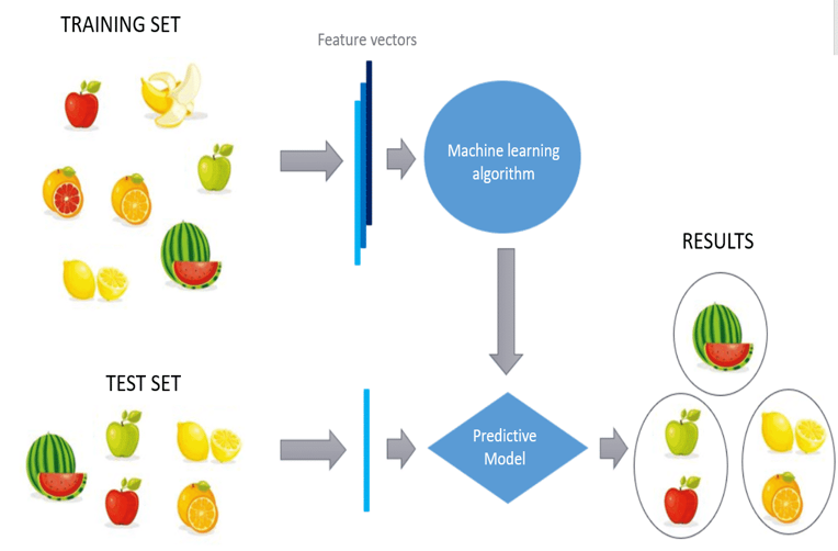
Learn from experience: Algorithms process training data to understand patterns and relationship.
Make predictions or decisions: Based on the patterns learned, the system can classify, predict or make decisions on new, unseen data.
Improve over time: As the system is exposed to more data, it refines its decision-making ability.
Machine learning is widely used in various fields, including finance, healthcare, marketing, and more for tasks such as fraud detection, customer segmentation, disease diagnosis, and recommendation systems.
Types of Machine Learning
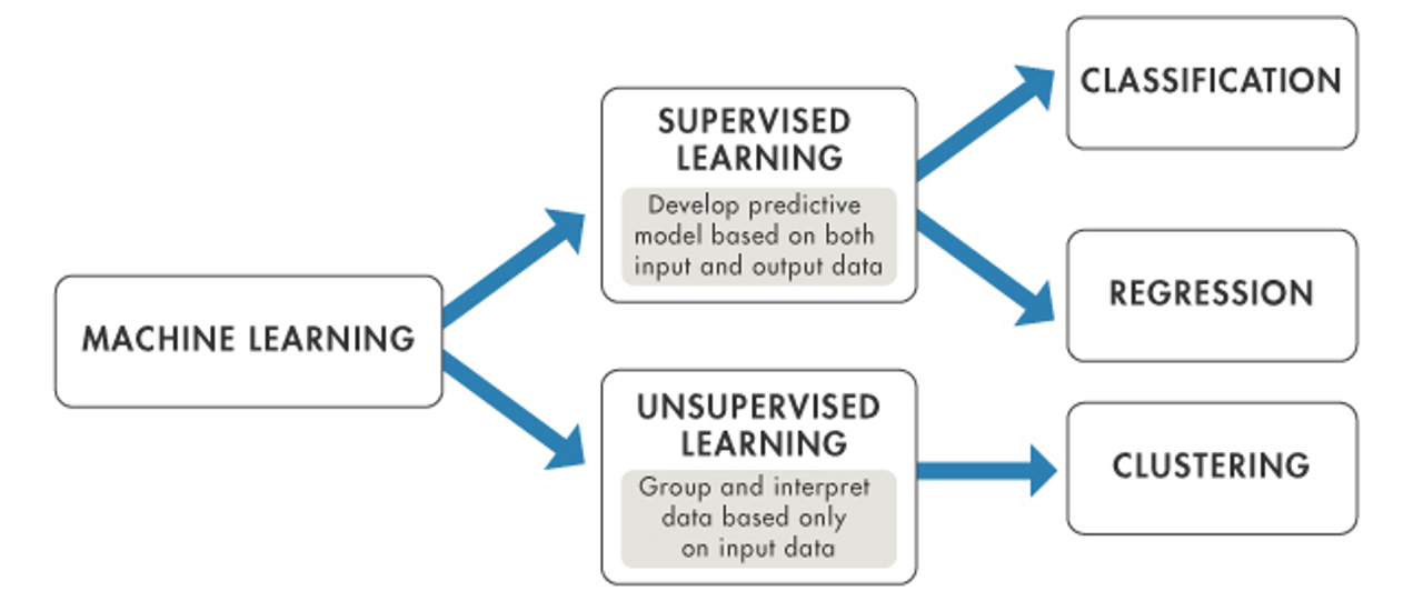
There are two main types of machine learning:
Supervised learning: The model is trained on labeled data, meaning that the input data is paired with the correct output. The model learns to predict the output from new inputs based on the relationships in the training data. Example include classification and regression tasks.
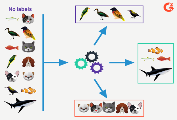
Unsupervised learning: The model is trained on unlabeled data, and the goal is to find hidden patterns or intrinsic structures in the data. Examples include clustering and dimensionality reduction.
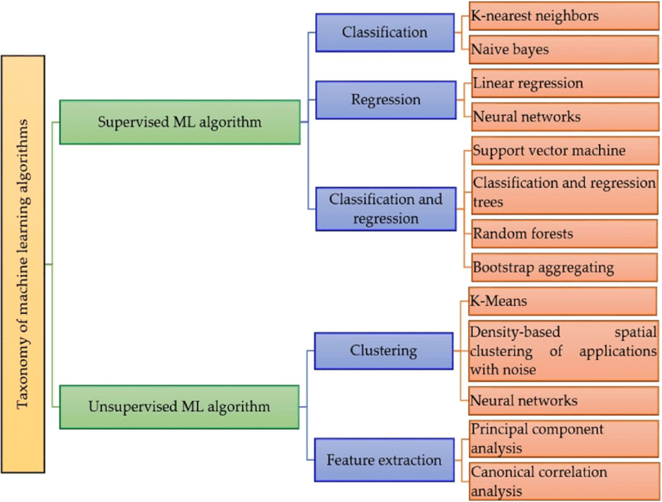
Taxonomy of Machine Learning algorithms
Supervised Learning
Supervised learning is the machine learning task of learning a function that maps an input to an output based on example input-output pairs. It infers a function from labeled training data consisting of a set of training examples.
In supervised learning, a dataset comprising of elements is given with a set of feature \(X_{1}\),\(X_{2}\) ,\(X_{3}\) ,…,\(X_{p}\) as well as a response or outcome variable \(Y\) for each element. The goal was then to build a model to predict \(Y\) using \(X_{1}\),\(X_{2}\) ,\(X_{3}\) ,…,\(X_{p}\).
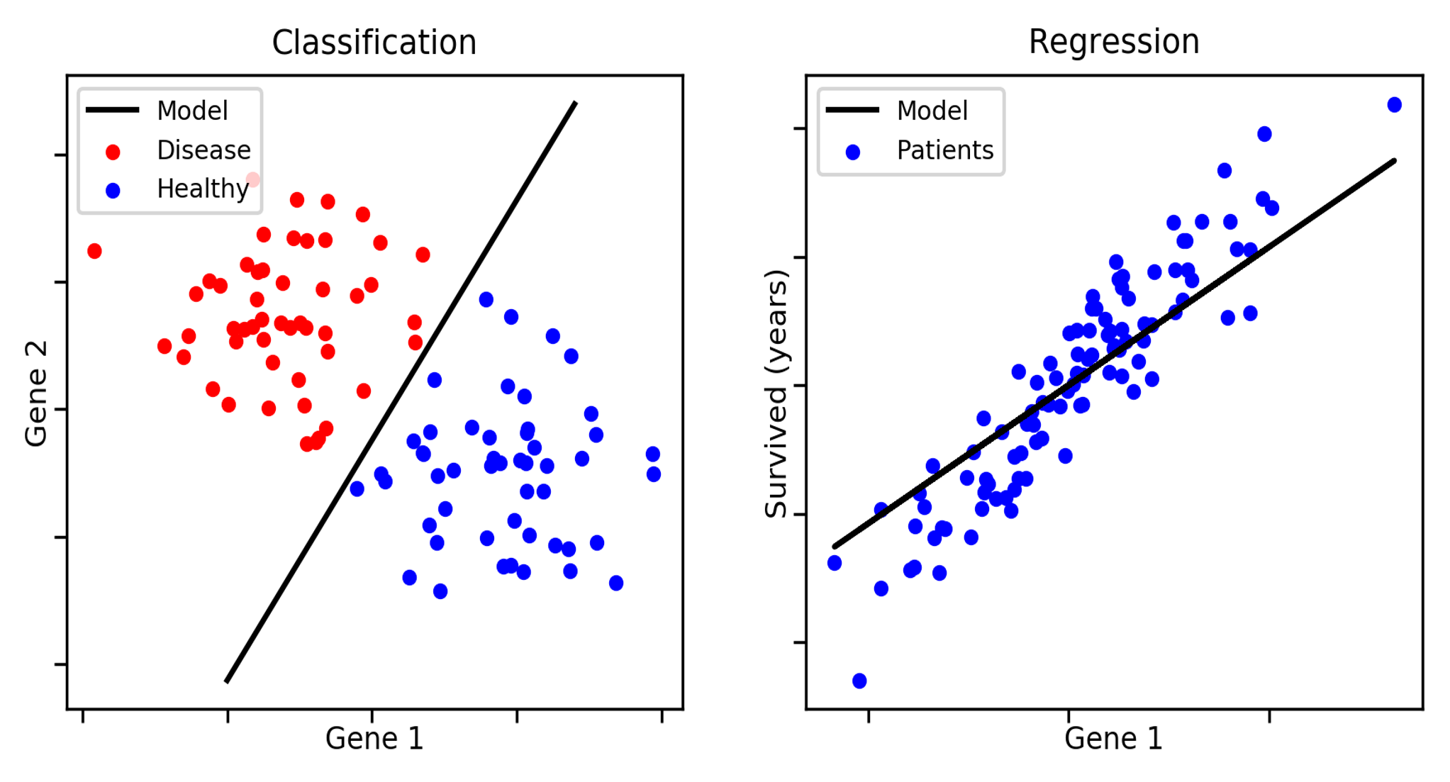
Classification
Supervised learning for classification: Attribution of a class or label to an observation by exploiting the availability of a training set (labeled data) or in other words Classification is a subcategory of supervised learning where the goal is to predict the categorical class labels (discrete, unordered values, group membership) of new instances based on past observations.
Unsupervised Learning
Unsupervised learning is a machine learning technique in which models are not supervised using training dataset. Instead, models itself find the hidden patterns and insights from the given data. It can be compared to learning which takes place in the human brain while learning new things. (Example: Clustering).
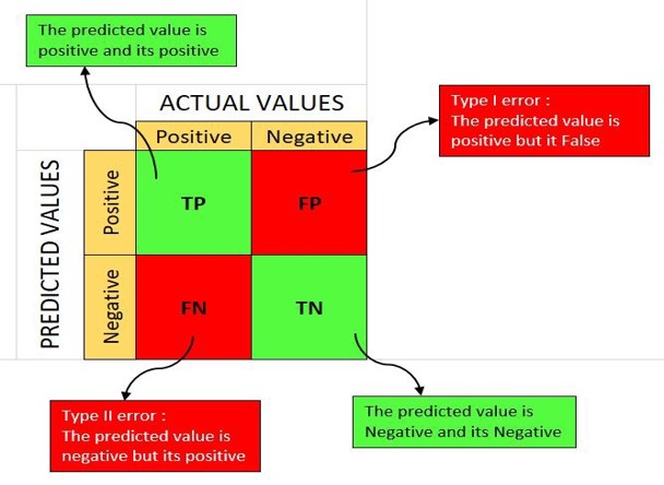
Classification Performance - Confusion matrix
A confusion matrix is a table that is often used to describe the performance of a classification model (or “classifier”) on a set of test data for which the true values are known.
Performance formula from confusion matrix:
\[
Accuracy = \frac{TP+TN}{TP+TN+FP+FN}
\]
\[
Sensitivity = \frac{TP}{TP+FN}
\]
\[
Sepecificity = \frac{TN}{TN+FP}
\]
Parameter vs Hyperparameters
The words “parameters” and “hyperparameters” are used a lot in machine learning, but they can be hard to understand. To optimize models and get better results, it is important to know the difference between these two ideas.
Parameters
Parameters are the internal configuration values that a machine learning model learns during the training process. They are adjusted based on the data the model is exposed to, allowing the model to fit the training data effectively.
For instance, in a linear regression model, the parameter include the coefficients associated with each feature. These coefficients represent the strength and direction of the relationship between the features and the target variable.
Model fitting and parameters
When talk about fitting a model, we refer to the process of adjusting the parameters to minimize the error in predictions. The fitted parameters are the output of this training process. In the context of machine learning, this is often referred to as “training the model”.
To illustrate, consider a simple linear regression model that attempts to predict a target variable based on one or more input features. The model’s output will include various statistics, such as:
Residuals: The differences between the predicted and actual values
Coefficients: The values that multiply each feature to produce the model’s output.
Statistical metrics: Such as R-Squared, which indicates how well the model explains the variability of the target variables.
These outputs are collectively referred to as model parameters. They are crucial for making predictions and are derived from the training data.
Hyperparameters
Hyperparameters differ significantly from model parameters. They are defined before the training process begins and dictate how the training will occur. Hyperparameters control the learning process itself rather than the model’s internal state.
For example, in a neural network, hyperparameters might include the learning rate, which determines how quickly the model updates its parameters during training, and the number of hidden layers, which defines the model’s architecture. These values need to be set prior to training and can significantly influence the model’s performance.
Defining hyperparameters
To identify which hyperparameters to set, you can look at the function calls used in your modelling process. Each function will have arguments that can be adjusted. For instance, in a linear model, the method of fitting can be considered a hyperparameter. Some common hyperparameters across different types of models includes:
Learning rate in neural networks.
Number of trees in a random forest
Regularization strength in regression models.
Batch size in stochastic gradient descent.
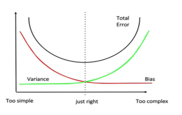
The importance of hyperparameter tuning
Hyperparameter tuning is a critical step in ensuring that a machine learning model performs optimally. Without proper tuning, a model may underfit or overfit the training data, leading to poor generalization to new, unseen data.
To understand the significance of hyperparameter tuning, consider the analogy of assembling a fantasy football team. Just as you would select the best combination of players to maximize your team’s chances of winning, you need to select the best combination of hyperparameters to maximize your model’s performance.
Naive Bayes
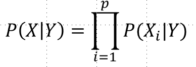
Naive Bayes is a probabilistic machine learning algorithm based on Bayes’ Theorem, which is used primarily for classification tasks. It is termed “naive” because it assumes that the features are conditionally independent given the class label, which may not always be true in real-world scenarios. Despite this strong assumption, Naive Bayes performs well in many applications, especially when dealing with text classification, spam filtering, and other tasks where the independence assumptions holds reasonably well.
The algorithm calculates the probability of each class based on the input features and classifies the new data point to the class with the highest posterior probability. Naive Bayes is particularly valued for its simplicity, speed, and effectiveness in situations where quick decisions are needed, and it is especially useful for large datasets with multiple features.
Objective of Naive Bayes for classification problems
The objective of Naive Bayes in classification is to build a model that can predict the class label of new, unseen data by estimating the conditional probability of each class given the input features. In the context of machine learning, this model:
Learns the relationships between the input features and the class labels from a training dataset.
Applies the learned probabilities to classify new data points.
Handles both categorical and continuous input variables, making it versatile for a variety of problems.
In this note, we will implement the Naive Bayes algorithm for classification using the caret pakcage in R. The caret package provides a unified interface for training various machine learning models, including Naive Bayes, allowing for easy implementation and comparison of model using consistent syntax.
The gene expression datasets of brain tissue was searched in the Gene Expression Omnibus (GEO) database using query: “Alzheimer* AND Homo sapiens” filtered by “Expression profiling by array” in August 2024. There are about 6,308 datasets found in search results. Out of these, 102 entries were sifted through. Finally, three datasets were chosen to be considered in this study since they were generated using the same platform (GSE5281, GSE48350, and GSE1297).
To understand mode about the dataset, we use str(). The str() function provides a summary of the dataframe, including the number of rows and columns, the data types of each column. This can be useful for quickly understand the structure and contents of a dataframe
str(data1)
'data.frame':   378 obs. of  31 variables:
 $ Group  : chr  "Control" "Control" "Control" "Control" ...
 $ PSEN1  : num  0.002109 0.0002 0.002062 0.000204 0.000121 ...
 $ APP    : num  0.001598 0.000126 0.001628 0.000179 0.000167 ...
 $ APOE   : num  0.001161 0.000208 0.001363 0.00017 0.000133 ...
 $ ACHE   : num  0.01227 0.00196 0.01331 0.0024 0.00229 ...
 $ TREM2  : num  0.005489 0.000683 0.005393 0.001216 0.000316 ...
 $ PSEN2  : num  0.02697 0.00227 0.02632 0.00299 0.00438 ...
 $ GRN    : num  5.68e-03 2.66e-04 5.69e-03 5.79e-04 4.82e-05 ...
 $ TNF    : num  0.007208 0.00058 0.007295 0.000548 0.000661 ...
 $ BDNF   : num  0.00815 0.000576 0.008177 0.002756 0.002627 ...
 $ MAPT   : num  0.002584 0.000215 0.002452 0.000219 0.000342 ...
 $ IGF1   : num  0.01843 0.00147 0.01676 0.00316 0.00562 ...
 $ BCHE   : num  0.006229 0.000999 0.007936 0.001008 0.000678 ...
 $ IL1B   : num  0.004271 0.001357 0.004417 0.000882 0.012836 ...
 $ GSK3B  : num  0.004883 0.000491 0.00445 0.000598 0.000917 ...
 $ BACE1  : num  0.003231 0.000205 0.003328 0.00032 0.000323 ...
 $ VEGFA  : num  0.002959 0.000114 0.002996 0.001265 0.001022 ...
 $ CLU    : num  5.34e-04 4.47e-05 5.51e-04 2.94e-05 3.38e-05 ...
 $ MAOB   : num  4.38e-04 6.87e-05 4.32e-04 4.34e-05 2.87e-05 ...
 $ ACE    : num  0.021382 0.002031 0.020632 0.000396 0.001923 ...
 $ CYP46A1: num  6.76e-04 5.56e-05 6.97e-04 7.97e-05 5.55e-05 ...
 $ CSF1R  : num  0.001596 0.000252 0.001821 0.000529 0.000051 ...
 $ SORL1  : num  1.14e-03 9.65e-05 1.16e-03 6.60e-05 8.95e-05 ...
 $ PPARG  : num  0.014888 0.001397 0.01649 0.000548 0.000855 ...
 $ NOS3   : num  0.009956 0.007751 0.010376 0.000925 0.000535 ...
 $ PLAU   : num  0.011568 0.000984 0.01246 0.001074 0.001138 ...
 $ APOC1  : num  0.001404 0.000156 0.001662 0.000696 0.000106 ...
 $ SNCA   : num  0.002948 0.000316 0.003019 0.000557 0.000507 ...
 $ GRIN2B : num  0.02261 0.00206 0.0219 0.00242 0.00265 ...
 $ INS    : num  0.0883 0.0123 0.0945 0.0106 0.0118 ...
 $ ABCA7  : num  0.0079 0.00171 0.008424 0.001703 0.000861 ...
The target variable for this dataset is Group, which consist AD patient and Control subject. Currently, the datatype for this variable is Character, we need to convert this variable to factor before proceed with the analysis.
This variable has been converted to factor datatype. There were 189 AD patients and 189 Control subjects in the dataset.
Checking any missing values
Before proceed with the analysis, we need to make sure our dataset is cleaned and free from any missing value. To check for missing value:
library(descriptr)ds_screener(data1)
----------------------------------------------------------------------
|  Column Name  |  Data Type  |  Levels  |  Missing  |  Missing (%)  |
----------------------------------------------------------------------
|     Group     |   factor    |AD Control|     0     |       0       |
|     PSEN1     |   numeric   |    NA    |     0     |       0       |
|      APP      |   numeric   |    NA    |     0     |       0       |
|     APOE      |   numeric   |    NA    |     0     |       0       |
|     ACHE      |   numeric   |    NA    |     0     |       0       |
|     TREM2     |   numeric   |    NA    |     0     |       0       |
|     PSEN2     |   numeric   |    NA    |     0     |       0       |
|      GRN      |   numeric   |    NA    |     0     |       0       |
|      TNF      |   numeric   |    NA    |     0     |       0       |
|     BDNF      |   numeric   |    NA    |     0     |       0       |
|     MAPT      |   numeric   |    NA    |     0     |       0       |
|     IGF1      |   numeric   |    NA    |     0     |       0       |
|     BCHE      |   numeric   |    NA    |     0     |       0       |
|     IL1B      |   numeric   |    NA    |     0     |       0       |
|     GSK3B     |   numeric   |    NA    |     0     |       0       |
|     BACE1     |   numeric   |    NA    |     0     |       0       |
|     VEGFA     |   numeric   |    NA    |     0     |       0       |
|      CLU      |   numeric   |    NA    |     0     |       0       |
|     MAOB      |   numeric   |    NA    |     0     |       0       |
|      ACE      |   numeric   |    NA    |     0     |       0       |
|    CYP46A1    |   numeric   |    NA    |     0     |       0       |
|     CSF1R     |   numeric   |    NA    |     0     |       0       |
|     SORL1     |   numeric   |    NA    |     0     |       0       |
|     PPARG     |   numeric   |    NA    |     0     |       0       |
|     NOS3      |   numeric   |    NA    |     0     |       0       |
|     PLAU      |   numeric   |    NA    |     0     |       0       |
|     APOC1     |   numeric   |    NA    |     0     |       0       |
|     SNCA      |   numeric   |    NA    |     0     |       0       |
|    GRIN2B     |   numeric   |    NA    |     0     |       0       |
|      INS      |   numeric   |    NA    |     0     |       0       |
|     ABCA7     |   numeric   |    NA    |     0     |       0       |
----------------------------------------------------------------------

 Overall Missing Values           0
 Percentage of Missing Values     0 %
 Rows with Missing Values         0
 Columns With Missing Values      0
There are no missing values in this dataset.
Step 2: Data Normalization
Before proceeding with analysis, it is the best practice to normalize the data to make sure all the variables in same scale. In this note, we will use min-max method to normalize the data.
# Min-max normalize all variables of mtcarsdata1_mm <-as.data.frame(scale(data1[-1],center =apply(data1[-1], 2, min),scale =apply(data1[-1], 2, max) -apply(data1[-1], 2, min)))data1 <-as.data.frame(cbind(data1[1], data1_mm))
Step 3: Splitting the dataset
In order to perform Machine learning classifier, we will split the dataset into training and testing set. Usually we will use \(\frac{2}{3}\) of the data for training set, and another \(\frac{1}{3}\) for testing set.
set.seed(123456) #set seed for reproducibilityU <- data1predictors <-names(U)[!names(U) %in%"Group"] #define all predictorslibrary(caret) #loading the caret library#Create splitting rules 70% for training and 30% for testing setinTrainingSet <-createDataPartition(U$Group, p=0.7, list=F) train<- U[inTrainingSet,]test<- U[-inTrainingSet,]x = train[,predictors] #predictors for training sety=train$Group #Outcome for training setx1=test[,predictors] #Predictors for testing sety1<-test$Group #outcome for test set
The dataset has been splited into training and testing set. There are 70% of the observations in training set, and 30% for testing set.
dim(train)
[1] 266 31
table(train$Group)
     AD Control
    133     133
In training set, we have 266 observations, 133 AD Patients and 133 Control subjects.
dim(test)
[1] 112 31
table(test$Group)
     AD Control
     56      56
In test set we have 112 Observations, 56 AD patients, and 56 Control subjects.
Step 4: Perform Naive Bayes classifier
First we need to set the cross validation method in tuning the hyperparameter for Naive Bayes. By using trainControl function in caret library, it allows use to specify how the model training process should be carried out, particularly during resampling and hyperparameter tuning. It controls aspects like:
Resampling method: techniques such as cross-validation, or bootstrapping to split data for performance estimation.
Performance metrics: Metric like accuracy, kappa, AUC (area under the ROC curve) that evaluate model performance.
Search Methods: Determines how to search for the optimal hyperparameters (eg: grid search or random search).
Key Arguments of trainControl.
Method:
“cv”: cross-validation, which splits the data into multiple folds (typically 10) and trains the model multiple times on different folds.
“boot”: Bootstrapping, which repeatedly samples the data with replacement and evaluates model performances.
“repeatedcv”: Repeated cross-validation, which performs cross-validation multiple times for more robust results.
Number: Specifies the number of folds for cross-valiadation or the number of bootstrap resamples. Typically used with “cv” or “repeatedcv” methods.
Repeats: If using repeated cross-validation, this argument sets how many times to repeat the cross-validation process.
summaryFunction: Defines the function used to compute performance metrics. For classification tasks “twoClassSummary”, you may want metrics like accuracy, kappa, or sensitivity.
search: Specifies the hyperparameter seach method, Common choices are:
“grid”: Grid search, which tests all possible combinations of specified hyperparameters.
“random”: Random search, which tests a random subset of hyperparameter combinations.
classProbs: Set to TRUE if you want the model to return predicted probabilities for each class. This is useful for models like Naive Bayes, where class probabilities are often used for decision making.
savePredictions: Controls whether the predictions on the resampled data should be saved. This is useful for comparing predictions later.
set.seed(123456) #set seed for reproducibilityfitControl <-trainControl(method ="cv", # cross-validationnumber =10, # number of folds (10-folds cv)summaryFunction = twoClassSummary, #Use accuracy, ROC, etc..classProbs =TRUE, #Enable probability predictionsearch ="grid", #Perform grid searchallowParallel = T, #parallel processing)
Step 5: Fitting the model - Naive Bayes
In fitting the machine learning classifier, there were many algotrithms offered by caret package. We can refer to this link to see the list of machine learning algorithms offered : https://topepo.github.io/caret/available-models.html
or we can simply use this function to see the list of available machine learning method :
names(getModelInfo())
1. Fitting the model using automated hyperparameter search
Now we can fit the model into caret library using train function.
library(tictoc) #to record the time tic() #begin record timeset.seed(123456) #set seed for reproducibilitynb_model <-train( Group ~ ., #Group as dependent and consider all variables leftdata = train, # using train dataset to learn from the datamethod ="nb", # using nb - naive bayes classifier.trControl = fitControl, #using pre-defined cross validation strategytuneLength =5#tuning for every spliting )toc() #stop record time
2.69 sec elapsed
Model summary
nb_model
Naive Bayes

266 samples
 30 predictor
  2 classes: 'AD', 'Control'

No pre-processing
Resampling: Cross-Validated (10 fold)
Summary of sample sizes: 240, 240, 238, 239, 240, 239, ...
Resampling results across tuning parameters:

  usekernel  ROC        Sens       Spec
  FALSE      0.6150405  0.1131868  0.9626374
   TRUE      0.6700972  0.5659341  0.6840659

Tuning parameter 'fL' was held constant at a value of 0
Tuning
 parameter 'adjust' was held constant at a value of 1
ROC was used to select the optimal model using the largest value.
The final values used for the model were fL = 0, usekernel = TRUE and adjust
 = 1.
Based on the model, we know that for my pc with 4 cores, i5 and 16gb RAM, it only tooks 2.71 second to complete the analysis. The model used 10 fold cross validation resampling method, to tune the hyperparameter. The final hyperparameter used were fL=0, use kernel = T, adjust = 1.
2. Fitting the model using automated hyperparameter search - Parallel processing
library(tictoc)tic() library(doParallel) #parallel processingcl <-makePSOCKcluster(3) #setting up the clusterregisterDoParallel(cl) #register cluster set.seed(123456) #set seed for reproducibilitynb_model2 <-train( Group ~ ., #Group as dependent and consider all variables leftdata = train, # using train dataset to learn from the datamethod ="nb", # using nb - naive bayes classifier.trControl = fitControl, #using pre-defined cross validation strategytuneLength =5#tuning for every spliting )nb_model2
Naive Bayes

266 samples
 30 predictor
  2 classes: 'AD', 'Control'

No pre-processing
Resampling: Cross-Validated (10 fold)
Summary of sample sizes: 240, 240, 238, 239, 240, 239, ...
Resampling results across tuning parameters:

  usekernel  ROC        Sens       Spec
  FALSE      0.6150405  0.1131868  0.9626374
   TRUE      0.6700972  0.5659341  0.6840659

Tuning parameter 'fL' was held constant at a value of 0
Tuning
 parameter 'adjust' was held constant at a value of 1
ROC was used to select the optimal model using the largest value.
The final values used for the model were fL = 0, usekernel = TRUE and adjust
 = 1.
stopCluster(cl)toc()
3.94 sec elapsed
By using parallel processing, it only took 4.7 second to perform the model. The hyperparameter tuning was done using 10-fold cross validation resampling. The final hyperparameter used were fL=0, use kernel = T, adjust = 1.
Warning
After using parallel processing, we need to unregister the foreach backend.
registerDoSEQ()
3. Fitting with manual grid hyperparameter search
Instead of using automated hyperparameter search from caret setting, we can also search our own hyperparameter setting.
Firstly, we need to know what hyperparameters available for the model. To know that we need to check the model specification:
modelLookup(model="nb")
  model parameter                label forReg forClass probModel
1    nb        fL   Laplace Correction  FALSE     TRUE      TRUE
2    nb usekernel    Distribution Type  FALSE     TRUE      TRUE
3    nb    adjust Bandwidth Adjustment  FALSE     TRUE      TRUE
Remember!
Each machine learning classifier have different hyperparameter! If we not sure what area of hyperparameter should be search, please only use automated searching. This function served for those who know the area to be searching.
#for NB, we set our hyperparameter search areaGrid =expand.grid(usekernel=TRUE,adjust=1,fL=c(0.2,0.5,0.8))set.seed(123456) #set seed for reproducibilitynb_model3 <-train( Group ~ ., #Group as dependent and consider all variables leftdata = train, # using train dataset to learn from the datamethod ="nb", # using nb - naive bayes classifier.trControl = fitControl, #using pre-defined cross validation strategytuneLength =5, #tuning for every spliting tuneGrid = Grid #Insert search area)nb_model3
Naive Bayes

266 samples
 30 predictor
  2 classes: 'AD', 'Control'

No pre-processing
Resampling: Cross-Validated (10 fold)
Summary of sample sizes: 240, 240, 238, 239, 240, 239, ...
Resampling results across tuning parameters:

  fL   ROC        Sens       Spec
  0.2  0.6700972  0.5659341  0.6840659
  0.5  0.6700972  0.5659341  0.6840659
  0.8  0.6700972  0.5659341  0.6840659

Tuning parameter 'usekernel' was held constant at a value of TRUE

Tuning parameter 'adjust' was held constant at a value of 1
ROC was used to select the optimal model using the largest value.
The final values used for the model were fL = 0.2, usekernel = TRUE and
 adjust = 1.
Step 6: Model Prediction
Once we have develop the model, we can do prediction by using test data.
We will use nb_model for this step.
Remember in step 3, we define x1 as all the predictors for test set
It is important to see how well the model performs for this dataset. We need to evaluate interms of accuracy, sensitivity, specificity, error rate and f-measure.
First, we need to get the confusion matrix from the predicted value.
Confusion Matrix and Statistics
predictions AD Control
    AD      30      19
    Control 26      37
Accuracy : 0.5982
95% CI : (0.5014, 0.6897)
No Information Rate : 0.5
P-Value [Acc > NIR] : 0.02337
Kappa : 0.1964
Mcnemar's Test P-Value : 0.37109
Sensitivity : 0.5357
Specificity : 0.6607
Pos Pred Value : 0.6122
Neg Pred Value : 0.5873
Prevalence : 0.5000
Detection Rate : 0.2679
Detection Prevalence : 0.4375
Balanced Accuracy : 0.5982
'Positive' Class : AD
Based on the performance evaluation, we can see that the accuracy of Naive Bayes model for the test set was 0.5982, sensitivity was 0.5357, and specificity was 0.6607.
To get full access of all performance measure we can call :
         Sensitivity          Specificity       Pos Pred Value
           0.5357143            0.6607143            0.6122449
      Neg Pred Value            Precision               Recall
           0.5873016            0.6122449            0.5357143
                  F1           Prevalence       Detection Rate
           0.5714286            0.5000000            0.2678571
Detection Prevalence    Balanced Accuracy
           0.4375000            0.5982143
Step 8: Variable Importance
By using caret package, we can get the list of variable importance.
The variable importance refers to a metric that ranks the features of a dataset based on their contribution to the prediction of the target variable. Depending on the model type, the method for calculating importance can vary.
This function lists only 20 most important biomarkers for AD.
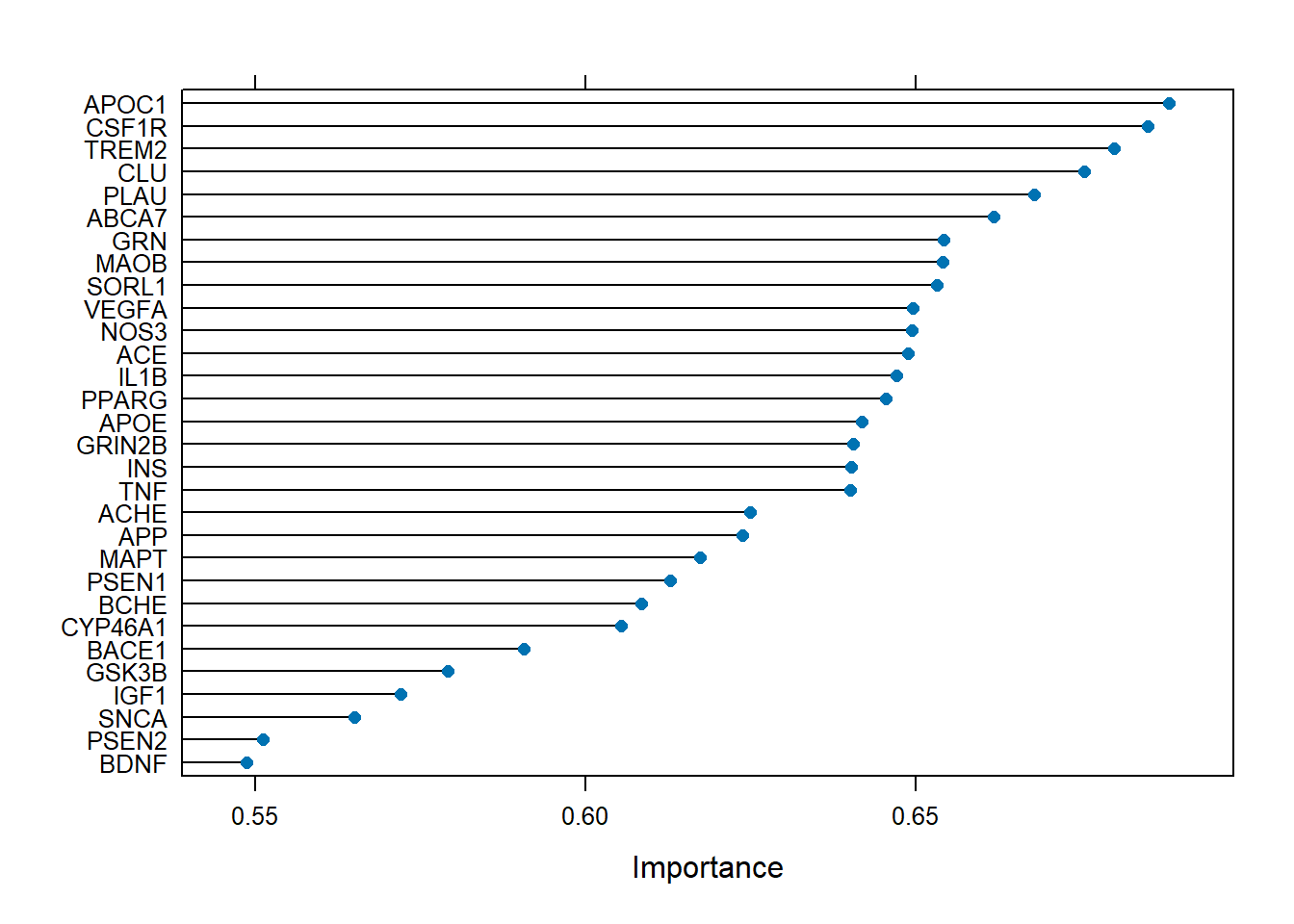
We can also plot the variable importance
plot(varImp(nb_model, scale=F))
Based on this, we can see that the APOC1 and CSF1R genes were the most important biomarkers for AD.
Dr. Mohammad Nasir Abdullah PhD (Statistics), MSc (Medical Statistics), BSc(hons)(Statistics), Diploma in Statistics,
Graduate Statistician, Royal Statistical Society.
Senior Lecturer,
Mathematical Sciences Studies,
College of Computing, Informatics and Mathematics,
Universiti Teknologi MARA,
Tapah Campus, Malaysia.